NC Accessibility Hub

Accessibility Requirements

Alternative Text

Alternative or alt text must be added to any non-text content — such as Images, Shapes, Graphics, and PivotCharts — that conveys a meaning or adds relevance to the Excel document.

Alt text may not be sufficient to describe the information displayed in complex images such as, graphs, and charts. In these cases, in-text descriptions can be used to provide a longer description. Alternatively, a description can be added to the cell behind the chart. The text can be hidden by changing the text colour to match the background. When the screen reader comes across the cell containing the chart, it will read the text description.

Adding Alt Text

There are 2 ways to add alt text.

Option 1

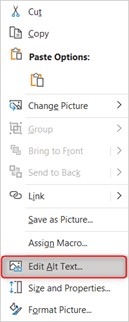
Right click on the object and select Edit Alt Text.

Option 2

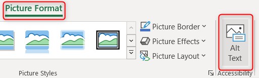
Select the object, then select Format > Alt Text.

Using the Alt Text Pane

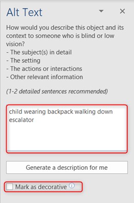
In the Alt Text pane, describe the object and its context. There is no need to add “image of …” before your description because the screen reader will indicate that it is an image. If the object offers no information or meaning, select the Mark as decorative checkbox screen readers will skip it.

Resources

This article by Microsoft will help you understand how to write effective alt text: Everything you need to know to write effective alt text (microsoft.com).

Back to Top

Hyperlinks

All hyperlinks should use descriptive text that accurately describes where the link leads to.

Descriptive Hyperlinks

To add a descriptive hyperlink:

1. Select the cell/text that you want to display as a hyperlink.
2. Right-click on the cell/text and click Link.
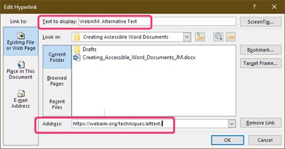
3. In the Insert Hyperlink box, type or paste the website URL in the Address box.
4. Add the descriptive text for your hyperlink in the Text to display box.

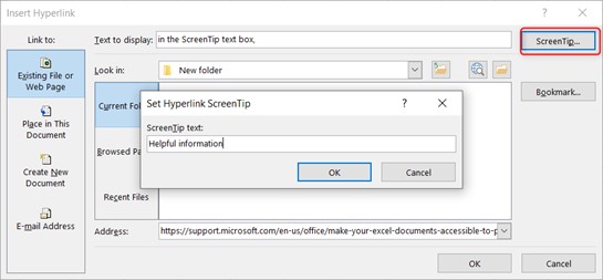
ScreenTips

A ScreenTip can also be added to provide more information. ScreenTips are small windows that display descriptive text when you rest the pointer on the hyperlink.

To add a ScreenTip:

1. Select the cell/text that you want to display as a hyperlink.
2. Right-click on the cell/text and click Link.
3. In the Insert Hyperlink box, select the ScreenTip button.
4. Type the text of the ScreenTip into the ScreenTip text box.

Colour and Contrast

The colours you choose are an important part of your content creation as it can impact people that you’re not even aware have disabilities such as those with colour-blindness or low-vision impairments.

Do not use colour alone to convey meaning or indicate importance. It’s better to indicate important concepts by using underlined or bolded text. Screen readers can detect these font features easily which will communicate the importance to the user.

It is essential that appropriate contrast exist between text and the background. Ensure there is sufficient contrast between text and the background you are using i.e., a contrast ratio of at least 4.5:1 for normal text and 3:1 for large text. A light background and dark text or dark background and light text will typically achieve good contrast, however a Colour Contrast Analyser can be used to make sure the contrast is sufficient.

Sheet Tab Title

Naming Sheet Tabs

All sheet tabs need to have a unique, meaningful title. This allows the reader to know what information is on each tab, making it easier to navigate.

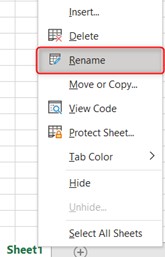
To name a sheet tab:

1. Right-click a sheet tab and select Rename.
2. Type a brief, unique name for the sheet, and press Enter.

Deleting Unused Worksheets

Remember to delete any unused worksheets. This will prevent screen reader users and keyboard navigators wasting time by opening a worksheet to determine if there is content in it.

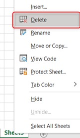
To delete a worksheet:

1. Right-click a sheet tab and select Rename.
2. Type a brief, unique name for the sheet, and press Enter.

Tables

To ensure accessibility, use simple tables structures i.e., do not merge cells, or manipulate other table elements. Format tables with headers. This helps to provide context and assist navigation of the table’s contents.

Adding Table Headings

There are two ways to add a table heading.

Option 1: Use Headers in an Existing Table

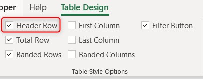
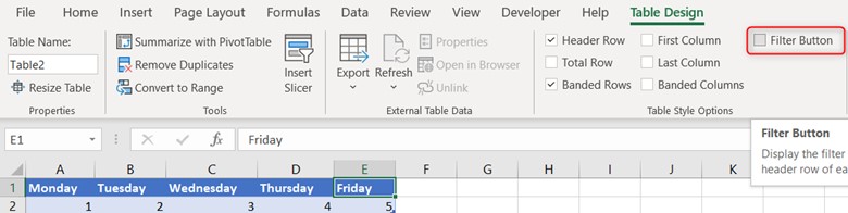
1. Click on the table.
2. On the Table Design tab, in the Table Style Options group, select the Header Row check box.
3. Type the column headings.

Option 2: Add Headers to a new table

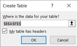
1. Select the cells you want to include in the table.
2. On the Insert tab, select Table.
3. Select the My table has headers check box.
4. Type new, descriptive names for each column in the table.

Note: Excel automatically applies a filter setting to a table. If you do not want to have a filter on your table, you can remove it by clicking on the table and going to the Table Design tab. Uncheck the filter button in the Table Style Options group.

Video and Audio

If video or audio are included in the worksheet, transcripts and/or captions must be included. To learn how to make your video accessible, review our Video Accessibility articles.

Document Properties

Descriptive Title

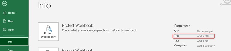
Adding a title to your document information allows screen reader users to preview document information without opening it. This can help limit the necessity of opening a document to determine if it’s the one they’re looking for. To add a descriptive title, click File > Info. The title is located under the Properties section.

Meaningful Filename

Be sure to use a meaningful name for your document. This will make is easier for users to find. For guidance on how to add meaningful filenames and descriptive titles to your documents check out the Video: Create accessible file names (microsoft.com).

Accessibility check

To check the accessibility of your Excel document, use the built in MS PowerPoint Accessibility Checker tool. The article Using the Accessibility Check in the Microsoft 365 Office Suite explains how to use this tool.

Accessibility Best Practices

Cell A1 

When a person uses a screen reader in Excel, the starting point is always cell A1. The screen reader will read across and then down the worksheet announcing the contents of each cell. When inserting a table, graphic, or chart, it’s important to create it in the first column. It’s tempting to view column one as a margin and insert your item in what seems to be visually centered on your page. However, if the cell has no content, it may lead the screen reader user to believe that the worksheet is empty.

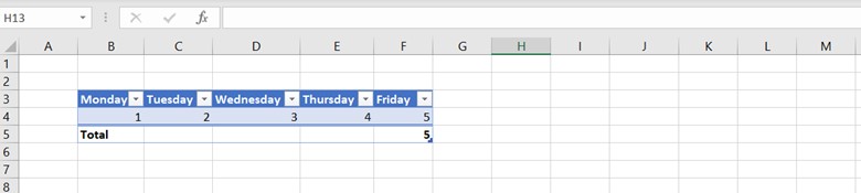
For example, in the screenshot below, the screen reader would read cells A1 through M1 first and then move onto cell A2. This could be confusing for screen reader users. In this example, if there was no preamble before the table, it would be best practice to create it beginning in cell A1.

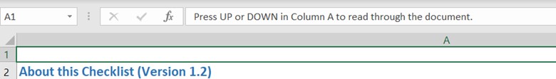
Alternatively, help text can be added to the in the first cell — A1 — that describes how to navigate the worksheet. A small font size or a font colour that is the same as the background can be used, so the text doesn’t show up visually but will still provide helpful context for screen reader users. For example, Press Up or Down in column A to read though the document.

Blank cells, rows, and columns

Avoid empty rows, columns, and cells as these might lead someone to believe there is nothing more in the worksheet. If any blank rows and columns are not necessary, simply delete them. If blank rows and columns are being used to create white space, resize the rows and columns to give them spacing that makes them readable. A common mistake is leaving column A blank to look like a margin.

If the above options are not appropriate, enter text explaining that they are blank. Some examples of appropriate text are: “No data” or “Intentionally Blank”. Use a font colour that is the same as the background so the text doesn’t show up visually but will still provide helpful context for screen reader users.

Unused cells, rows, and columns

It can be helpful for screen reader users and people with cognitive disabilities to hide any unused cells, rows, and columns in a worksheet. This makes the worksheet less cluttered and helps readers to focus on important information. It also helps screen readers users as it lets them know that they are not missing any content. 

To hide unused cells, rows, and columns:

1. Select the column/row beneath the sheet’s last used column/row.
2. To select every column, press Ctrl +Shift+ Right Arrow.
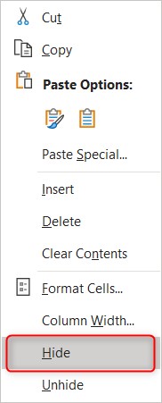
3. Right click and select hide.
4. To select every row, press Ctrl +Shift+ Down Arrow.
5. Right click and select hide.

Tip

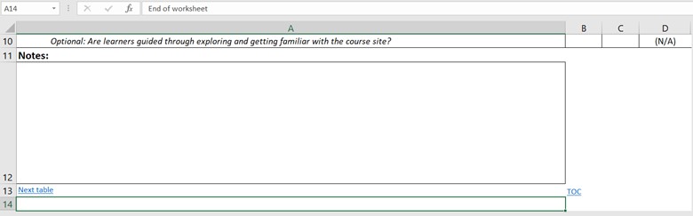
Add a label at the end of the worksheet to let users know that there is no other content beyond that point. Use a font colour that is the same as the background so the text doesn’t show up visually but will still provide helpful context for screen reader users.

Merged or Split cells

Merging or splitting cells can make navigating difficult for people using assistive technologies. Merged cells can be used in a title of a table but should not be used in the data part of table. Use a simple and straightforward structure for displaying content.

Excel Forms

If you are creating a form in Excel, there are a few other tools that can help with accessibility:

• Setting the print area: Set or clear a print area on a worksheet (microsoft.com)
• Providing an input messages about your form fields: Video: Input and error messages (microsoft.com)  
• Locking cells so only certain cells can be edited: Lock cells to protect them (microsoft.com)
• Protecting workbook to prevents user from deleting, copying worksheets, or renaming tabs: Protect a workbook (microsoft.com)

Additional Resources